Introduction
The
macroscopic behavior of the
TCP congestion avoidance algorithm
by Mathis, Semke, Mahdavi & Ott in
Computer Communication Review, 27(3), July 1997, provides a short and useful
formula for the upper bound on the transfer rate:
Rate <= (MSS/RTT)*(1 / sqrt{p})
where:
Rate: is the TCP transfer rate or throughputd
MSS: is the maximum segment size (fixed for each Internet path, typically
1460 bytes)
RTT: is the round trip time (as measured by TCP)
p: is the packet loss rate.
Note that the Mathis formula fails for 0 packet loss. Possible solutions are:
- You assume 0.5 packets were lost. Eg. assume you send 10 packets each
30 mins for 1 year then 48 (30 min intervals in day) * 10 packet *365 days = 175200 pings or a loss rate of 0.5/175200 = 0.00000285.
- You take the Padhye estimate (see bwlow) for 0 packet loss, i.e. Rate = Wmax / RTT.
The default Linux Wmax is 12k8Bytes (see Linux Tune Network Stack (Buffers Size) To Increase Networking Performance).
An improved form of the above formula that takes into account
the TCP initial retransmit
timer and the Maximum TCP window size, and is generally more accurate for
larger (> 2%) packet losses,
can be found in:
Modelling TCP throughput: A simple model and its empirical
validation by J. Padhye, V. Firoiu, D. Townsley and J. Kurose,
in Proc. SIGCOMM Symp. Communications Architectures and Protocols
Aug. 1998, pp. 304-314. The formula is given below (derived from eqn 31 of
Padhye et. al.):.
if w(p) < wmax
- Rate = MSS * [((1-p)/p) + w(p) + Q{p,w{p}}/(1-p)] /
- (RTT * [(w{p}+1)]+(Q{p,w{p}}*G{p}*T0)/(1-p))
otherwise:
- Rate = MSS * [((1-p)/p)+ wmax+Q{p,wmax}/(1-p)] /
- (RTT * [0.25*wmax+((1-p)/(p*wmax)+2)] +
(Q{p,wmax}*G{p}*T0)/(1-p)])
Where:
We have assumed the number of packets acknowledged by a received ACK is 2
(this is b in the Padhye et. al. formula 31)
wmax is the maximum congestion window size
w{p} = (2/3)(1 + sqrt{3*((1-p)/p) + 1} from eqn. 13 of Padhye et. al.
substituting b=2
- Q{p,w} = min{1,[(1-(1-p)3)*(1+(1-p)3)*(1-(1-p)(w-3))] /
- [(1-(1-p)w)]}
G{p} = 1+p+2*p2+4*p3+8*p4+16*p5+32*p6
from eqn 28 of Padhye et. al.
T0 = Initial retransmit timeout (typically this is suggested by
RFCs 793 and 1123 to be 3 seconds).
Wmax = Maximum TCP window size (typical default
for Solaris 2.6 is 8192 bytes)
If you are tuning your hosts for best performance then also read
Enabling High Performance Data Transfers on Hosts
and
TCP Tuning Guide for Distributed Application on Wide Area Networks. Also
The TCP-Friendly
Website summarizes some recent work on congestion control for non-TCP based
applications in particular for congestion control schemes that maintain the
arrival rate to at most some constant over the square root of the packet loss
rate.
A problem with both formulae for 0 packet loss is that the throughput depends on RTT which may change by little from year to year for a host pair with terrestrial wired links. Thus the formulae start to fail for long term trends unless one knows the Wmax as a function of time for such pairs of hosts. Unfortunately this is typically only known by the system administrators and may change with time.
Measurement of MSS
On June 7-8, 1999, we measured the MSS between SLAC and about 50
Beacon sites by sending
pings with 2000 bytes and sniffing on the wire to see the size of the
response packets. Of the 48 Beacon site paths pinged all except 1 responded
with an MSS of 1460 bytes (packet size of 1514 bytes as reported by the
sniffer), and the remaining 1
(nic.nordu.net) was unreachable.
Validation of the formula
Between May 3 and May 15, 1999, Andy Germain of the Goddard Space Filght
Center (GSFC) made measurements of TCP
throughput between GSFC and Los Alamos National Laboratory (LANL).
The measurements were made with a modified version of ttcp
which, every hour, sent data from GSFC to LANL for 30 seconds and then measured
the amount of data transmitted. From this a measureed TCP throughput was
obtained. At the same time Andy sent 100 pings from GSFC to LANL and measured
the loss and RTT. These loss and RTT measurements were plugged into the formula
above to provide a predicted throughput.
We then plotted the measured TCP throughput (ttcp) and the predicted (from ping)
throughput and the results are shown in the chart below.
It can be seen from the variation between day and night that the link is
congested. Visually there is reasonable agreement between the predicted
and measured values with the predicted values tracking the predicted ones.
Note that since only 100 pings were measured per sample
set, the loss resolution was only 1%. For losses of < 1% we set the loss
arbitrarily to 0.5%.
To further evaluate the agreement between the predicted and measured values we
scatter plotted the predicted versus the measured values as shown in the chart
below.
It can be seen that the points exhibit a strong positive correlation with an
R2 of about 0.85. In this plot points with a ping loss of < 1% are omitted.
How the Formula behaves
Using the above formula with an MSS of 1460 bytes, we can plot the throughput as a function
of loss and RTT as shown in the chart below for the range RTT from 0.25ms (typical LAN RTTs)
to 650ms (typical geostationary satellite speed). If one takes the speed of light in fibre
as roughly 0.6c or msec = alpha * 100km where empirically alpha ~0.4 accounts for
non direct paths, router
delays etc. then the distances corresponding to 10, 50, 100, 250, 500, 1000, 2500, 5000, 10000, 25000km are
0.25, 1.25, 2.5, 6.25, 12.5, 25, 62.5, 125, 250, 625 msec.
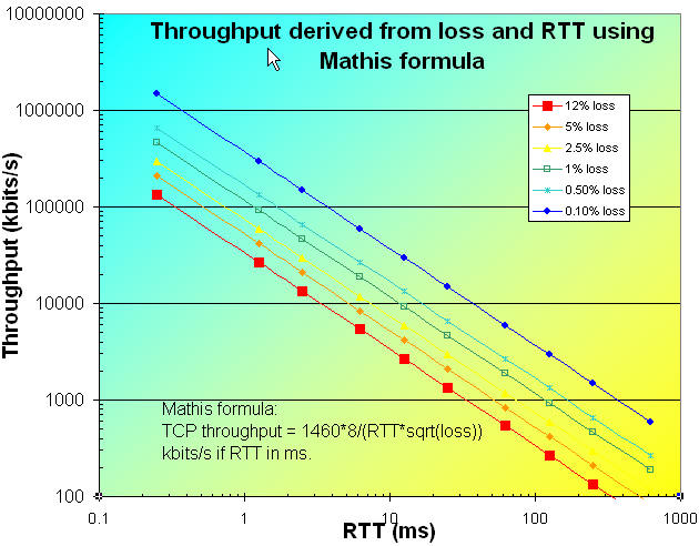
In the above chart the lines are colored according to
the packet loss quality defined in
Tutorial on Internet
Monitoring. Given the difficulty of reducing the
RTT, the importance of minimizing packet loss is apparent.
If we consider how the packet loss is improving month-to-month
(see
Tutorial on Internet monitoring at SLAC) then
the loss appears to be improving by between 2% and 9% / month. Applying
the above formula, fixing
the RTT at 100 msec. and starting with an initial loss of 2.5% we get
the throughputs shown in the following figure for various values from
0% to 10% improvement/month:
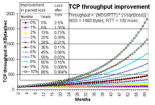
In order to facilitate understanding, the table on the left of
the chart above, shows the yearly improvement in loss and the loss at the
end of three years.
Using the formula with long term PingER data
Given the historical measurements from PingER of the packet loss and RTT we can
calculate the maximum TCP bandwidth for the last few years for various groups of
sites as shown in the figure below. The numbers in parentheses in the legend
indicate the number of pairs of monitor-remote sites included in the group
measurement. The percentages to the right show the improvement per month, and
the straight lines are exponential fits to the data.
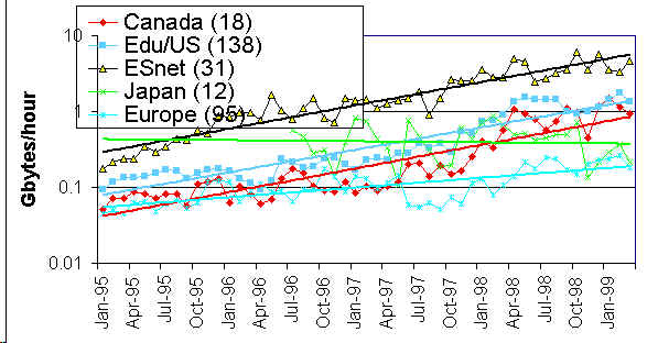
Another way of looking at the data is to show the Gbytes that can be transmitted
per hour. This is shown in the chart below between ESnet and various
collections of sites.
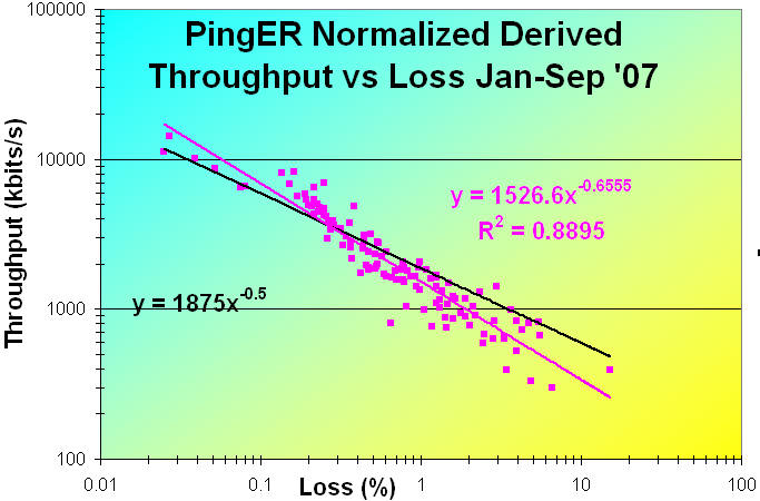
The figure below shows the Normalized Derived PingER Throughput measured from SLAC to
countries of the world from january through September 2007 as a function of the packet loss.
Normalization is of the form:
Normalized Derived TCP throughput(AKA Normalized Rate) =
(Minimum_RTT(Remote country)/Minimum_RTT(Monitoring Country)) * Rate
The correlation is seen to be strong with R2 ~ 0.89,
and goes as 1526.6 / loss0.66.
Also shown is a rough fit for the 129 countries with observed data minimizing
X=Sum(Theory-Observation)/Theory)2) where Theory = beta/sqrt(loss),
beta = 1875 and X= 12.43.
Correlation of Derived Throughput vs Average RTT and Loss
The correlation of Derived Throughput is stronger versus Loss than versus
Average RTT. This can be seen in the images below:
| Derived Throughput vs Average RTT |
Derived Throughput vs Loss |

|

|
[
Feedback |
Reporting Problems
]
Les Cottrell

